Showing posts with label AuroraWatchNet. Show all posts

Tuesday, 28 October 2014

FTDI all-in-one serial converter, programmer, switch


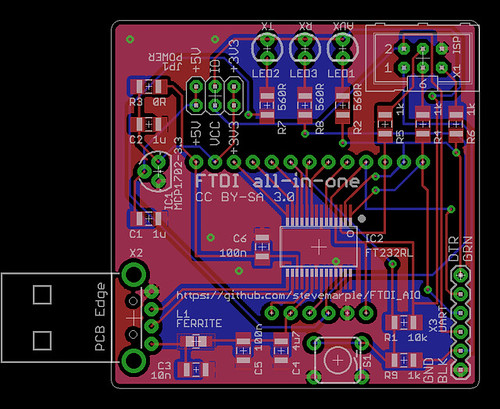
FTDI all-in-one
FTDI all-in-one PCB layout.

There are a multitude of FTDI converters and breakout boards available but none of them exactly fitted my needs so this is my version tuned to suit my requirements. I'm publishing the design files in the hope they are useful for others. Like the Sparkfun FTDI Basic Breakout and the Adafruit FTDI Friend it uses the FTDI FT232R but there are a number of differences, for instance it has a USB type A connector to plug directly into a USB host port.

Serial converter

The FTDI AIO provides a serial adaptor with the standard 6 pin FTDI pinout (TX, RX, CTS, DTR, VCC, and GND). A jumper block enables the VCC pin to be switched between +3.3V and +5V. A separate jumper enables the logic levels of the TX, RX, DTR and CTS signals to be set for +3.3V or +5V operation. The Sparkfun FTDI Basic Breakout can also be switched between +3.3V and +5V operation but does not allow for independent selection of VCC and the logic levels. This means when the Sparkfun FTDI Basic is set for +3.3V operation it's not compatible with the standard FTDI cables, which always supply +5V to the VCC pin. Whether that's a good thing or a bad thing depends on your needs; the FTDI AIO gives you both options.

AVR ISP programmer

Programming AVR microcontrollers, even with just a small bootloader, can be painfully slow and normally I'd use the AVR Dragon. There are situations however where it would be useful to have a low-cost USB programmer. A bit-banging AVR programmer is easily made and Adafruit has an excellent tutorial which explains how to do this.The FTDI all-in-one makes this convenient by providing the standard AVR ISP header. The defacto AVR standard is that the VCC pin is set to the same voltage as the logic-level signals. Unfortunately this practice isn't followed by +3.3V Arduino boards which always set VCC to +5V. For the widest compatibility the AVR ISP VCC pin can be set to either +3.3V or +5V with the logic levels of the !RESET, MISO, MOSI and SCK signals independently configured to either  +3.3V or +5V.

On-board +3.3V voltage regulator

One of the features of the FT232R is that it has a built-in +3.3V regulator. This was used by older Arduinos to provide a +3.3V supply. However the current capability is limited to just 50mA which in many cases is not sufficient to power a microcontroller and all of its peripherals. The FTDI all-in-one can include an on-board voltage regulator with 250mA current output which should be sufficient to power an Arduino and several shields.

Auxiliary switch and LED

One of the key features I wanted was the ability to add an auxiliary switch and LED to the Raspberry Pi. Although the Pi has GPIO the AuroraWatchNet magnetometers normally have a radio fitted to this connector, which prevents it being easily used for other purposes. I worked around this by wiring a switch and LED to a Sparkfun FTDI Basic Breakout but I wanted a single PCB which plugged directly into one of the Pi's USB sockets.

Why would you want a switch? There are probably many uses. Mine is that I run one of the AuroraWatchNet magnetometers and I wanted a way to conveniently signal when I am going to cut the grass, or make some other magnetic disturbance in the garden.The data logging software, which runs on a Raspberry Pi, checks for the existence of a file which signals data quality might be bad. When the file is present data is logged to a separate set of files which aren't used by the AuroraWatch UK alerts system. While it's no bother for me to create the file by logging into the Pi I needed something simpler for other members of the family, so I wanted to wire up a switch. A separate daemon monitors the serial port to detect if the switch is pressed, if so the LED is turned on and the semaphore file created. If the switch is pressed again the file is removed and the LED turned off. The LED actually tracks the state of the file being present so it is possible to override the monitor process by creating or removing the semaphore file by other means.

Breakout board

All of the GPIO pins from the FTDI FT232R are conveniently broken out to pads spaced at 0.1" pitch. Also included are pads for the filtered +5V supply obtained from USB and +3.3V from the on-board regulator (if fitted, otherwise from the FT232R's built-in regulator).

Why use the FT232R?

Given the recent controversy regarding FTDI and Windows drivers you might wonder why I am using the FT232R instead of some other device. I'd probably prefer to use the Microchip MCP2200 USB UART converter for this application as it works well with my Calunium Arduino clone and it is available in a SOIC package which is easier to work with at home. Unfortunately its not possible to read the CTS line with the USB CDC driver which rules it out.

Open-source hardware

The Eagle PCB design files are available on Github and are licensed under the Creative Commons Attribution-ShareAlike 3.0 (CC BY-SA 3.0) license.

The PCB layout is not yet tested, although I did breadboard and test all of the functionality. I'll be sending the design off for manufacture in the next few days, it's likely I'll have a few boards spare.

Update: the first boards have been assembled and tested; all features work as planned. The bit-banging AVR ISP programmer is even slower than I feared, taking about 10 minutes to read the 4Kb EEPROM on the Atmel ATmega1284P on one of my Calunium boards.

Monday, 24 March 2014

Power over ethernet (PoE) magnetometer and cloud detector

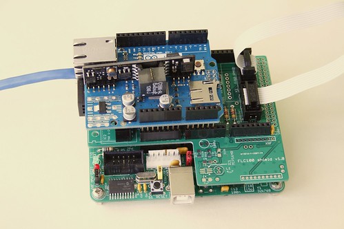
Combined magnetometer and cloud detector
Combined magnetometer and cloud detector.


To improve the performance and stability of the AuroraWatchNet magnetometers I recently began experimenting with a power over ethernet (PoE) version. With restrictions on power consumption lifted considerable performance improvements are possible. As a result I have developed the magnetometer hardware specifically to support a power over ethernet version. Another instrument I've been developing is a cloud detector. This too should benefit from a power over ethernet version. One problem I encountered was with dew settling on the sensor but fitting a heater is incompatible with battery-powered operation. Since both the magnetometer and cloud detector use almost the same hardware I decided to design an Arduino-compatible 'shield' that could be used to support both systems.

Combined magnetometer and cloud detector hardware

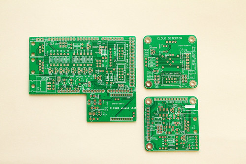
Combined magnetometer and cloud detector PCBs
Printed circuit boards for the sensor shield (left), the IR or humidity sensor (top right)
and fluxgate magnetometer (bottom right). Click for annotated version.
The complete system requires six circuit boards (five for the wireless version). The first is the microcontroller board, I use my Calunium Arduino clone. I hope that in future it will be possible to use an off-the-shelf Arduino Mega2560 instead but the current firmware relies on Calunium's real-time clock to generate the hardware interrupts which control the sampling interval. There is also a sensor shield, the Arduino Ethernet shield (omitted on the battery-powered wireless version), and one board for each of the sensors (fluxgate magnetometer, IR temperature and humidity).

The sensor shield is based on the existing design and retains the option of battery-powered operation with radio communication. The magnetometer sensor and analogue-to-digital converter must be powered at 5V, which requires a level-shifting circuit when the microcontroller is powered from 3.3V, which is the case when operating from batteries. For power over ethernet use the microcontroller must also operate at 5V for compatibility with the Arduino Ethernet shield so the level shifting is not required. It is kept however as it provides buffering between the two circuit boards; 1.5m is a considerable distance for an I2C bus. The cloud detector uses a non-contact infra-red temperature sensor operating at 3.3V so a level-shifting circuit is required for PoE operation where the microcontroller is connected to 5V. (I've ignored the fact that a 5V version of the sensor exists since it isn't readily available in the UK). The sensor shield allows a humidity sensor to be connected so that estimates of the clear sky and cloudy sky temperatures can be made. As before, an on-board LM61 temperature sensor monitors the system temperature. The new sensor shield also adds a header to fit an Embedded Adventures lightning sensor module. I don't have one of these at the moment so I can't be certain it will work and there is no software support for it in the existing firmware. Fitting it at the same time as the cloud detector sensors will require long break-away headers to be soldered to the bottom of the lightning sensor module.

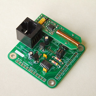
Fluxgate magnetometer sensor PCB
Fluxgate magnetometer sensor mounted on its sensor PCB.
Click for annotated version.

The fluxgate sensor is fitted on its own PCB which contains the analogue to digital converter. For PoE operation a linear voltage regulator is used to convert from 9V to the 5V supply it requires. For battery operation a MAX619 DC-DC charge pump boosts the battery voltage to 5V. Almost all of the temperature variation can be removed by placing the PCB at the bottom of a 1m length of soil pipe. The pipe is buried to a depth of 0.85m with its axis vertical. In the magnetometer-only system the microcontroller, sensor shield and ethernet shield (or batteries for the wireless version) are fitted onto a wooden frame to hold them into the top part of the tube. Positioning the rest of the system away from the fluxgate sensor helps to avoid unwanted effects from any ferro-magnetic components (such as the batteries), it also aids access and enables wireless data transmission.

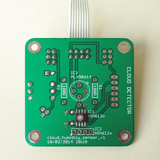
Humidity sensor PCB
Honeywell HIH6131 humidity sensor mounte on its sensor PCB.
The same PCB design is also used for the MLX90614 IR temperature sensor.
Click for annotated version.

The enclosure design used for the magnetometer isn't suitable for the cloud detector so the prototype cloud detector used a standard IP65 rated box, with the IR temperature sensor pointing upwards to view the sky. The humidity sensor was fitted above a breather hole in the bottom of the box. This concept will continue to be used for the cloud detector; the IR temperature sensor and humidity sensor are fitted to separate PCBs in the top and bottom of the box. To minimise costs the IR temperature and humidity sensors use the same PCB design. The mechanical design of the cloud detector part is something I'd like to improve upon, particularly to reduce the number of PCBs used. However the differing sensor requirements may prevent this.

For a combined system I plan to use the soil pipe to house the fluxgate sensor but locate the rest of the electronics in a separate box following the design of the prototype cloud detector.

Does it work?

I've not yet deployed a system outside but testing indicates the new printed circuit boards work as intended when used in power over ethernet mode. Battery-powered operation on this new version has not yet been tested.

Design files

The design files (hardware, firmware and software) are open source and can all be downloaded from the Github repository. A PDF version of the user manual describing how to construct and operate the magnetometer can be downloaded from http://aurorawatch.lancs.ac.uk/manual.pdf. At the time of writing only instructions to build the original FLC100 shield are included. Instructions to build the combined sensor shield described above will be added in due course.


Wednesday, 12 February 2014

Performance comparison of power over ethernet (PoE) and battery magnetometers

Introduction

I've been working to improve the performance and stability of the AuroraWatchNet magnetometers. It's apparent that both measurement noise and stability are considerably improved when the sensor is powered continually. Unfortunately with the sensor powered continually the batteries last for only a few weeks. I have therefore been testing a power over ethernet (PoE) version of the magnetometer. The hardware is essentially the same but the addition of the Arduino Ethernet shield requires the microcontroller to operate from 5V. Operating voltage is easily changed on my Calunium microcontroller board. With the power restrictions lifted the sampling interval can also be reduced. The test system has been operating reliably for almost two months, sampling every 5 seconds. With some minor configuration changes sampling every second is possible although I am not convinced the trade-off in measurement noise is worthwhile.

Performance comparison

Below is a plot comparing one hour of data from the new power over ethernet system with two of the existing battery-powered wireless models already in operation. The PoE system is on the same site as LAN1 but located nearer parked cars. I chose this period because it was free of man-made disturbances. I adjusted the baselines so that the plots overlap.Only the H component of the magnetic field is shown.

Power over ethernet compared with existing AWN magnetometers
Click for larger version.

The graph shows that the power over ethernet version has much smaller measurement errors; it can probably operate with ~0.1nT accuracy compared to ~10nT for the battery-powered version. It's such an improvement that I found the measurement accuracy was being limited by the available resolution of the analogue-to-digital converter. The battery-powered versions derive the sample value from the median of 15 samples (taken as a burst over 4 seconds) to reduce noise. To improve the resolution for the PoE version it operates by taking the mean of 15 samples. Further improvement to the resolution may be possible by taking advantage of the programmable gain amplifier that is built into the analogue-to-digital converter.

Let's see how it compares against some observatory-grade measurements. The plot below shows the same interval but this time uses data from the British Geological Survey magnetometers at Eskdalemuir and Hartland. I obtained the data from the SAMNET data archive at Lancaster University, where the data has already been converted into HEZ magnetic coordinates. AuroraWatchNet also operates with HEZ magnetic coordinates, although usually the E and Z sensors are not present. As before, the baselines have been adjusted so that the plots overlap.


PoE magnetometer compared with BGS magnetometers
Click for larger version.


The similarity between the different traces is striking. Some differences are to be expected since Eskdalemuir is approximately 140km north of Lancaster and Hartland is 350km SSW of Lancaster. This interval is interesting because it shows Pi2 pulsations, starting at about 01:15 and ending around 01:30. The period of the pulsations are about 90 to 120 seconds.

Conclusions

For a home-built citizen-science magnetometer which probably costs 25 times less than its observatory grade cousin I'm very happy with its performance. The detection of Pi2 pulsations means a low-cost magnetometer can now notify of substorm onset, not just the arrival of geomagnetic storms. A network of such devices has interesting possibilities for the study of magnetic field line resonances.

You might wonder why anyone would want to buy an observatory grade instrument, there are good reasons. At present I am relying on the sensor manufacturer's calibration, whilst an observatory grade instrument would be supplied with an official calibration certificate. The observatory instrument would also have better long-term baseline stability, lower temperature variation and higher cadence. Calibration is an issue I hope to tackle at a later date. For space-weather monitoring only short-term variations are of interest and
the better performance provided by an observatory system may not be needed.

Data credits

The Sub-Auroral Magnetometer Network data (SAMNET) is operated by the Space Plasma Environment and Radio Science (SPEARS) group, Department of Physics, Lancaster UniversityHartland and Eskdalemuir data is provided courtesy of the British Geological Survey.


Sunday, 27 October 2013

Magnetometer progress report: link indicator LED

I recently added a new feature to the magnetometer remote sensor unit firmware. To help indicate when it is within radio communication range of the base unit an LED is turned on at the start of a message communication. When the sensor unit receives the acknowledgement from the base unit of successful message receipt the LED is switched off. In normal operation the LED should blink briefly every 30 seconds, after each sampling interval. If the LED remains on it indicates a problem with the radio link. For the initial installation the sampling time can be reduced to 5 seconds for to obtain faster feedback of whether communication is successful or not.

Improvements for battery-powered operation

Indicating link errors by using an LED is convenient during installation but the power wasted after installation is not compatible with battery-powered operation. To save power the LED is used only the first 15 minutes of operation. Only user-initiated reset actions (power on or reset switch pressed) cause the LED to be used, resets from by the watchdog timer or brown-out detector are ignored. The cause of the reset is detected by examining the microcontroller's status register (MCUSR).


Communication timeout feature added

I've also added a timeout which detects when communication has been lost for an extended period. The microcontroller system is rebooted in the hope that the error is recoverable. Loss of communication, along with low battery status, can also be sensed and reported by running the latest version of the data plotting software on the Raspberry Pi. If either error is detected a message can be sent via email, Twitter or Facebook.


Saturday, 19 October 2013

Cloud detector: a review of progress so far

The hardware

My cloud detector has been running outside for over 5 months now. Overall I'm very pleased with how it works. The battery-powered hardware is based on the AuroraWatchNet magnetometer design, which uses my own Calunium microcontroller development board. The remote sensor board and fluxgate sensor are omitted. I've added a Melexis MLX90614 non-contact infra-red thermometer to measure the sky temperature. Clear skies should give low temperatures whilst clouds are expected to have warmer temperatures, although still colder than the ambient temperature. The MLX90614 also outputs the sensor temperature, which should be close to the ambient temperature. I also added a Honeywell HIH-6131-021 humidity sensor which has an I2C interface. Do not confuse with the similar sounding version which has an SPI interface! The HIH-6130 also provides and ambient temperature measurement. To avoid direct contact with water the humidity sensor is placed at the bottom of the enclosure with a hole underneath to expose it to air. This hole also functions as a breather hole and ensures that the internal pressure matches atmospheric pressure. Since this hole was drilled there have not been any more incidents of water ingress.

The Calunium board is running a firmware is a modified version of the magnetometer firmware. It communicates with the Raspberry Pi data logger using an 868MHz radio link, with the same signed communication protocol used by AuroraWatchNet. This means I can use the data recording software from AuroraWatchNet. It also inherits the signed over-the-air firmware update capability. In principle it should be possible to combine both magnetometer and cloud detector functions in one unit.

I started off using the 90°  field-of-view version of the non-contact IR thermometer but later switched to theMLX90614ESF-DCH-000-TU-ND variant which features a 12° field of view. Its greater height meant it was easier to fit into the cable grommet housing. However I think the FOV is too narrow and I plan to switch back to the original sensor when I have time.

Data processing

The data processing and plotting now uses the auroraplot library for Python, which I developed to process the AuroraWatchNet magnetometer data. On the graphs I plot the sky temperature measured by the non-contact IR thermometer and the ambient temperature measured by the humidity sensor. For monitoring purposes I also plot the sensor temperature of the IR thermometer (marked as "detector temperature"); this should be similar to the ambient temperature but its exposed position makes it more likely to undergo solar heating and radiative cooling. For good measure I also plot the system temperature, which is measured by an LM61 temperature sensor connected to the ATmega1284P's analogue to digital converter. This measurement is noisy but useful to check the system doesn't overheat on sunny summer days.

The plan is to estimate the upper and lower bounds that I would expect for the sky temperature, and from that derive an estimate of the cloud cover. I initially expected that with complete cloud cover the sky temperature would match that the lifted condensation level, which I estimate using the ambient temperature and relative humidity. I soon saw temperatures higher than the LCL temperature. Research literature indicates that the clouds can act as a mirror at long IR wavelengths and thus the expected temperature should include an effect of ground temperature too. On the plots this is shown as the effective cloud temperature. The clear sky temperature is derived from results found in research literature but none of the equations tried so far have been a great match. Other researchers have fitted parameters for their specific location (including altitude) by comparison with visual measurements. I have yet to try this but daily measurements are made at the nearby Hazelrigg Weather Station. The graphs are too cluttered for production use but help me to understand what is happening.

Example plots

Below are a selection of plots. You can see the entire archive (from 2013-07-14) at http://aurorawatch.lancs.ac.uk/testing/cloudwatch/test2/.

cloud_detector_20130903
Cloud detector data for 2013-09-03. The asterisk (*) indicates derived parameters (ie not directly measured).
The figure above include most of the effects that can be identified. After midnight there is thick cloud, which later clears for short periods. At around 0300 UT I think it must have rained, the sky temperature is almost identical to the detector temperature and the variability is much reduced. Whilst the sensor is wet no sensible conclusions about cloud cover can be drawn. At about 0700 UT the sensor clears of water and the sky temperature falls indicating clearer skies. The rest of the day is dry, with heavy cloud cover until 1400 UT. At around 1700 UT the skies are completely clear. The clear sky estimate is too low for this time. At 2000 UT the clouds return, with some clear patches.


Cloud detector, 2013-09-28
Cloud detector data for 2013-09-28 showing the effect of clear skies.
The figure above shows an almost completely cloud-free day. The higher variability in the sky temperature measurements between 1200-1600 UT corresponds to similar effects in the humidity data (shown below); both are direct measurements made by different sensors.

Relative humidity, 2013-09-28
Humidity data for 2013-09-28. Notice how the higher variability occurs at the same times as the sky temperature measurements.

Dew

During summer operation dew has not been a problem but now that the nights are colder I have noticed effects which I believe are due to the formation of dew on the sensor. In the first plot below the sky temperature apparently rises from around 2230 UT. The rise is smooth and during this period the ambient temperature is falling, which overnight is often a sign of clear skies. After midnight (second plot) the sky temperature increases slightly before falling sharply around 0630 UT. Sunrise on this day was 0622 UT.

Cloud detector, 2013-10-05Cloud detector, 2013-10-06
This pair of plots is believed to show dew formation on the sensor.


Conclusions

I know from the informal comparisons with visual cloud cover that I regularly make the cloud detector does generally work very well. It does not function during wet periods. As anticipated dew is becoming a problem during the colder nights and a dew heater will be required for reliable winter operation. Future development will be to add a heater, which will need a wired connection to the cloud detector. Once a wired connection is made the radio link appears superfluous so I plan to investigate the options for power-over-ethernet. The Arduino ethernet shield is one possibility, although its compatibility with 3.3V operation has not been established.

Thursday, 26 September 2013

Auroraplot: data processing software for AuroraWatchNet

With the dispatch of the AuroraWatch schools' magnetometers imminent I have implemented a  Python  toolkit to process the data. The numpy and matplotlib modules are used extensively. The toolkit provides an API to load data and perform various processing actions on it, such as plotting data. The concept is influenced by my previous Multi-instrument Analysis toolbox for Matlab. In addition to the loading and processing of magnetic field data auroraplot allows other data types to be added later.

Loading data

Data can be loaded with arbitrary start and end times very simply:

md = ap.load_data('AURORAWATCHNET', 'LAN1', 'MagData',
                  np.datetime64('2013-09-20T12:00:00+0000'),
                  np.datetime64('2013-09-21T12:00:00+0000'))


In this case the selected portion of data crosses midnight and two data files must be loaded, concatenated and trimmed to get the desired time range. This is performed automatically by auroraplot, the user need not be concerned with the format of the files or where they are located. It is even possible for the files to be downloaded on-the-fly using FTP or HTTP transfer protocols.

load_data returns an object (of type MagData) to the user containing the actual magnetic field data and various other metadata, such as a timestamp for each sample and the data units. Each object can store more multiple data channels but all data points must share the same timestamps, be of the same type and share the same units. Therefore it is not possible to store operating temperatures (units °C) in an object holding magnetic field strength (units tesla). The operating temperature data can be accessed as:

td = ap.load_data('AURORAWATCHNET', 'LAN1', 'TemperatureData',
                  np.datetime64('2013-09-20T12:00:00+0000'),
                  np.datetime64('2013-09-21T12:00:00+0000'))


Battery voltage (data type VoltageData) can be accessed in a similar same way.

Plotting data

High-level plot functions enable the data be be plotted very simply, for the magnetic field data loaded previously

md.plot()


will produce a matplotlib figure with a title and the axes labelled with the correct units. Temperature and voltage data are plotted in the same way.

I have created some tools to make working with numpy's datetime64 and timedelta64 objects more convenient, including rounding functions (round, ceil and floor) which round to an interval. They are useful for finding the start of an hour, or the end of a day. I have also created Locator and Formatter classes to sensibly label time axes using datetime64 times and timedelta64 intervals. Tick marks are located on the nearest second, minute, hour, day, month or year boundary (or multiple thereof) depending on the time interval being displayed. Thanks to matplotlib's structure the labels are automatically regenerated with the most appropriate time units when a plot is zoomed.

Other operations

Quiet-day curves

Other operations include the generation of quiet-day curves. These are the curves from which we measure geomagnetic activity and are of critical importance for AuroraWatch UK. There are are not flat but have a daily variation caused by the equatorial electrojet. The empirical algorithm selects the days (typically 5) with the least geomagnetic activity. A truncated Fourier series is used to guarantee that the quiet-day curves are cyclic, with the start and end points having the same magnitude and slope. This is essential otherwise our rolling plots would show up the discontinuities in the QDC at midnight, and would falsely cause step changes in the geomagnetic activity. An example QDC is shown below.

qdc
Quiet-day curve for magnetometer at Lancaster ,UK. This is derived from recorded data
and clearly shows the Sq current system caused by the equatorial electrojet.

From this we can see that even on a geomagnetically quiet day we would expect a 30nT variation in field strength seen by the magnetometer. The AuroraWatch threshold for minor geomagnetic activity is 50nT so this shows the importance of using a quiet-day curve instead of a flat line when calculating geomagnetic activity.

Stack plots

Stack plots (also called magnetograms) are a convenient representation for magnetic field data from a set of magnetometers separated in latitude.Data from the northernmost instruments is placed at the top and that from the southernmost at the bottom. An example stackplot is shown below:

20130920
Stackplot showing data from two Lancaster stations and from Ormskirk.
The magnetometer at Ormskirk is operated by the Met Office as part of a test. The stackplots will be more interesting as the network grows.

Open source

The source code is available under a BSD-type license from Github.You will need python, along with the numpy (version 1.7), matplotlib and scipy python modules.auroraplot has been tested under Debian Linux (64 bit version) and Raspbian on the Raspberry Pi.


Monday, 20 May 2013

Cloud detector progress

Microcontroller and radio communications

To minimise the time and effort required to test the cloud detector concept I am following the approach used for the AuroraWatchNet magnetometer system and reusing as much hardware from it as possible. The MLX90614 non-contact infra-red temperature sensor is located outside. To minimise the infrastructure requirements the sensor unit is battery-powered and transmits its data over a bi-directional radio link. The sensor is controlled by one of my Calunium v2 microcontroller development boards. I'm using a pair of RFM12B radio modules operating at 433MHz to emulate a transparent serial connection. One is fitted on  the Calunium board and the other radio module is connected to a Raspberry Pi via my RFM12B shield. The Pi records the data and is responsible for uploading it for general access. I am also reusing most of the AuroraWatchNet firmware, which means I already have signed data communications and the capability to deploy over-the-air firmware updates - quite a good starting position for a new project!

Waterproofing the sensor

The biggest challenge I expect to face with this project is waterproofing the sensor. Although it is hermetically sealed there is no easy way to deploy it outside. As explained in a previous post, only a few materials are transparent to long-wave infra-red emissions and the better ones are toxic, water-soluble or expensive. I am therefore trying to avoid covering the sensor window and instead keep the electrical contacts dry. My first attempt was to drill a hole in the box and attach the sensor with silicone sealant. The mechanical fixing lacked strength and I wasn't convinced I had completely sealed around the sensor. To make matters worse I ended up with sealant on the sensor window which had to be cleaned off before it set. Another approach was required.

The new approach is to fit the sensor inside a cable gland. Before doing so I had to attach wires to the sensor connectors and insulate with heat-shrink sleeving. The result is shown below.


The next step is to fit the sensor in the cable gland before fitting the cable gland to the box.


The other end of the wires can then be soldered. For the prototype the wires are soldered to a small piece of stripboard. The stripboard has two pull-up resistors for the I2C bus and a decoupling capacitor. There is also an IDC connector to link the board to the unused JTAG interface. This was the easiest way to connect to a stock Calunium v2 board. For the lowest power operation the sensor is powered from logic-level output and I am using software I2C so all connections can be grounded when the sensor is not in use. The real-time clock on Calunium is connected the the hardware I2C interface on the microntroller and can be operated independently of the sensor.


The box and cable gland are rated IP65. Hopefully the result will be waterproof  

Results

The sensor is now deployed outside and reporting back to the Raspberry Pi base station. The transmitted packets are logged by the Raspberry Pi but as yet I don't have a convenient way to extract the ambient and object temperatures for analysis. That is the next task.


Sunday, 3 March 2013

Three-axis sensor unit for AuroraWatchNet

Three-axis magnetometer sensor unit
Three-axis sensor unit. The RJ-45 connector is for power and I2C data signals, not Ethernet.

AuroraWatchNet is a network of magnetometers for auroral alerts and citizen science. Whilst the  magnetometer is intended to function with one single-axis FLC100 sensor from Stefan-Mayer Instruments I have designed the system to support 3-axis operation by mounting 3 sensor boards at 90° to each other using just standard right-angle PCB connectors. This approach avoids the requirement for external mounting hardware which would be expensive to manufacture.

The power supply (a charge-pump DC-DC converter), temperature sensor and RJ-45 connector are fitted to just one circuit board. It is possible to use only one analogue-to-digital converter (ADC) but given their low cost it was presumed they would be fitted to all boards to enable simultaneous sampling of all 3 axes. The MCP3424 converter was chosen because eight options are available for the I2C address, thus jumpers can be fitted to select a unique address for every ADC on the I2C bus. This converter also features 4 input channels. All magnetometer outputs and the temperature sensor are connected to each ADC so that the spare channels can provide some redundancy in case of an ADC failure. The SYNC connectors of all sensors are linked to synchronise their excitation frequencies.

Several single-axis units have been built and one is in active use by AuroraWatch UK. The photograph above shows the first three-axis unit to be built. Initial testing indicates it functions as intended but the performance of 3 simultaneously-powered sensors in close proximity is yet to be established.


Sunday, 10 February 2013

The importance of brown-out detection

The batteries expired in one of the AuroraWatchNet test magnetometers this week. I was expecting that to happen since the magnetometer wasn't operating in its low-power mode and the battery voltage from the two 1.5V alkaline cells had been hovering around 2V for some time. The Atmel ATmega1284P microcontroller is actually powered at 3.3V using a boost power supply. What I didn't expect was for the system to not start after replacing the battery. I could tell xboot was working since the LED flashed 3 times as usual after the reset button was pressed. After that the LED stayed on but nothing else happened, not even the start-up debug messages from the serial port. I guessed the flash program memory had somehow got corrupted.

I used the AVR Dragon to extract the contents of the flash memory (avrdude -P usb -c dragon_jtag -p atmega1284p -U flash:r:flash.img:r) and compared it against the saved raw image file using the linux split and cmp commands. Sure enough, three pages of flash memory were set to 0xFF, probably from some erroneous page clear operation. Brown-out detection was disabled by the fuse settings to save power. Big mistake! What I think happened was as the voltage dipped below its valid range the microcontroller started executing random commands, including 3 SPM page clears, one of which was the first page of flash which holds the interrupt vector table. Valid execution was doomed.

What I should have done was to enable brown-out detection in the fuses, 2.7V seems the most appropriate setting for an 8MHz clock and 3.3V operation. To save power during sleeping the brown-out detection can be disabled with a call to sleep_bod_disable(). Lesson learned!

Sunday, 13 January 2013

Magnetometer progress report

About AuroraWatchNet

I am developing a simple, low-cost, battery-powered magnetometer for auroral alerts and citizen science. It is intended to be wireless to allow easy installation, a unique feature as far as I am aware. The magnetometer uses my own Calunium micro-controller board, which is an Arduino clone based on the ATmega1284P micrcontroller. Data is sent via a radio link to a Raspberry Pi base station which will then forward the data to AuroraWatch UK. I am hoping to deploy a network of such magnetometers in 2013 to enable AuroraWatch UK users to contribute data to improve the service. If you want to track the development then follow @aurorawatchnet on Twitter. 

The first AuroraWatchNet magnetometer is currently running in my garden. The environment is not ideal as I can see disturbances from cars and even the garage door being opened but it is convenient for testing and representative of what to expect from user-contributed data. I have been comparing the results from our SAMNET magnetometers with the AuroraWatchNet prototypes and generally the results are very encouraging given the difference in cost between the two systems. Now I can plot the AuroraWatchNet magnetometer data in the standard AuroraWatch UK style, using the same Octave code. Below is a comparison of today's plots. 

AuroraWatch UK

The data is taken from SAMNET's Lancaster magnetometer. The X axis is time and the Y axis shows the magnetic field strength in the direction of magnetic North (H component) in nanotesla (nT) relative to an unrecorded baseline. This exact plot appeared on AuroraWatch UK. We would normally expect cleaner data but our Lancaster site has recently been experiencing some interference.

SAMNET data from Lancaster, as used by AuroraWatch UK

AuroraWatchNet test magnetometers

The plots below correspond to the same time interval as the plot above. The first plot is from my garden magnetometer.

AuroraWatchNet data from near Lancaster.

The Y axis again records magnetic field strength but this time it is the absolute field. This magnetometer is operating in power-saving mode, turning off the sensor when not needed. This slightly increases the noise level but I hope will give one year of operation from two D cells.

Another AuroraWatchNet magnetometer has been deployed almost adjacent to the SAMNET magnetometer we already use for AuroraWatch. In this system the magnetometer sensor is continually powered, resulting in reduced noise levels. The alignment with magnetic North is only approximate. 


AuroraWatchNet data from the Lancaster University field station.

Conclusion

The AuroraWatchNet magnetometers are sufficiently sensitive and stable to make useful contributions for auroral detection and citizen science. My experience with the garden magnetometer suggests that in many cases performance will be limited by the noise at the site, rather than the magnetometer.

Monday, 8 August 2011

Test magnetometer results

Test magnetometer
Magnetometer electronics in their temporary housing.

On Friday I deployed my magnetometer to the same site used by SAMNET for the Lancaster magnetometer. I knew that several coronal mass ejections (CMEs) were due to impact the Earth's magnetosphere. The predictions were correct, on Saturday AuroraWatch UK issued an amber alert. Below is a comparison of the data from my test magnetometer and the SAMNET magnetometer.

Test magnetometer (top-panel) and the D component from SAMNET's Lancaster magnetometer (bottom panel).
Sensor temperature for the same period.
The results are encouraging even though at present the test magnetometer isn't calibrated, and the orientation is only approximately aligned with the magnetic east component ("D"). The baseline differences can be ignored as SAMNET does not make full-field measurements, just variations from a fixed baseline. I haven't measured it yet but the test sensor has a large temperature coefficient; if the FGM-1 behaves in the same way as the FGM-3 then I expect it to be around 25nT/°C. The graph shows the temperature over the same period varied from 16.5°C to 30°C.

Clearly some kind of temperature stabilisation is going to be needed. One option is to bury the sensor. Another is active temperature control, but care will be needed to ensure that DC currents for the heater do not affect the magnetic field being measured!